X-ray Diffraction Course — Tutorial 02
FWHM of X-ray Peaks
Understanding Peak Broadening — From Crystallite Size to Microstrain Analysis
Tutorial at a Glance
Series: X-ray Diffraction Hub | Tutorial: 08 of 12 | Prerequisites: Basic XRD knowledge, Bragg's Law, Unit Cell and Lattice Parameters
Reading time: 40 minutes | Includes: FWHM definition, peak broadening mechanisms, Scherrer equation, Williamson-Hall analysis, instrumental broadening, worked examples, MCQs, key takeaways
SEO Keywords: FWHM XRD, full width at half maximum, peak broadening analysis, Scherrer equation crystallite size, Williamson-Hall method, microstrain XRD, X-ray diffraction peak width measurement, instrumental broadening
Table of Contents
1. Introduction to Peak Broadening
Welcome to this comprehensive tutorial on the Full Width at Half Maximum (FWHM) of X-ray diffraction peaks. If you have completed our earlier tutorials on Bragg's Law and crystal structure, you know that X-ray diffraction produces sharp, well-defined peaks that correspond to specific crystal planes. Each peak appears at a specific angle 2θ determined by Bragg's Law: nλ = 2d sinθ.
But look more carefully at any real XRD pattern, and you will notice something important: the peaks are not infinitely sharp. They have width. They are broadened. This broadening is not noise or experimental error — it carries critical information about the material's microstructure. The width of a diffraction peak, quantified by its FWHM, tells us about the size of crystallites, the presence of internal strain, and the degree of structural perfection in the material.
The Central Question This Tutorial Answers
When you measure an XRD pattern and see peaks with measurable widths, what causes that broadening? How do we extract quantitative microstructural information — crystallite size, microstrain, defect density — from the peak width? And how do we do this correctly, accounting for instrumental effects and physical limitations?
This tutorial will build your understanding progressively. We start with the concept of FWHM itself — what it is and how to measure it. We then explore the three main physical causes of peak broadening: small crystallite size, microstrain, and instrumental limitations. We introduce the famous Scherrer equation, which relates peak width to crystallite size, and the more sophisticated Williamson-Hall analysis, which separates size and strain contributions. Finally, we apply these concepts to real-world materials characterization problems.
By the end of this tutorial, you will be able to measure FWHM from an XRD pattern, apply the Scherrer equation to calculate crystallite size, construct a Williamson-Hall plot to separate size and strain effects, and critically evaluate your results with awareness of the method's limitations.
2. What is FWHM?
2.1 Formal Definition
Definition: Full Width at Half Maximum (FWHM)
The Full Width at Half Maximum (FWHM), denoted as β, is the width of a diffraction peak measured at half of its maximum intensity. It is expressed in degrees 2θ (or radians for calculations) and represents the angular range over which the diffracted intensity is at least 50% of the peak maximum.
Let me translate this definition into concrete terms using a simple analogy.
The Mountain Peak Analogy
Imagine you are looking at a mountain from a distance. The mountain has a peak — the highest point. Now imagine a horizontal line drawn exactly halfway between the base of the mountain and the summit. This line intersects the mountain at two points: one on the left slope, one on the right slope. The horizontal distance between these two intersection points is analogous to the FWHM. It measures how "wide" the mountain is at half its height.
In an XRD peak, the "height" is the diffracted intensity (counts per second), the "summit" is the maximum intensity Imax, and the "halfway height" is Imax/2. The width between the two points where the intensity equals Imax/2 is the FWHM.
Mathematically, if a diffraction peak has its maximum intensity Imax at angle 2θpeak, then the FWHM is the angular difference between the two 2θ positions where the intensity drops to Imax/2. For a deeper understanding of peak width measurements, this concept is used across spectroscopy and diffraction techniques:
where the intensity at 2θleft and 2θright is exactly Imax/2.
2.2 How to Measure FWHM
In practice, measuring FWHM from an experimental XRD pattern involves several steps:
- Identify the peak maximum: Locate the angle 2θpeak where the diffracted intensity reaches its maximum value Imax. Modern XRD software can do this automatically by fitting the peak to a mathematical profile function.
- Calculate half-maximum intensity: Compute Imax/2. This is the intensity level at which you will measure the peak width.
- Find the half-maximum positions: Moving left from the peak center, find the angle 2θleft where the intensity first drops to Imax/2. Moving right from the peak center, find 2θright where the intensity drops to Imax/2 on the other side.
- Calculate FWHM: Subtract: β = 2θright − 2θleft. This is your measured FWHM in degrees.
- Convert to radians if needed: Many equations (like the Scherrer equation) require FWHM in radians. Convert using: β(radians) = β(degrees) × π/180.
Peak Fitting for Accurate FWHM
In professional XRD analysis, we rarely measure FWHM by manual inspection. Instead, we fit the peak to a mathematical profile function — typically a Gaussian, Lorentzian, or Voigt (Gaussian-Lorentzian convolution) function. The fitting software then reports the FWHM parameter directly from the fitted curve. This approach is more accurate because it reduces noise effects and handles overlapping peaks more reliably.
For a Gaussian peak: βGaussian = 2.355 × σ, where σ is the standard deviation of the Gaussian.
For a Lorentzian peak: βLorentzian = 2Γ, where Γ is the half-width at half-maximum parameter.
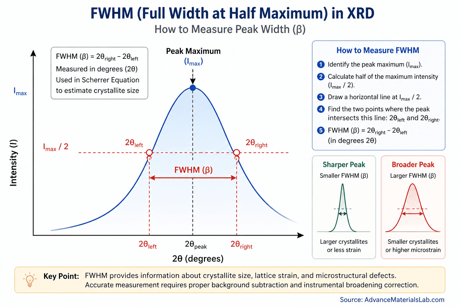
Fig. 1: Visual demonstration of FWHM measurement on an X-ray diffraction peak. The diagram shows the peak intensity profile with the maximum intensity (Imax) at the peak center, the half-maximum intensity level (Imax/2) marked by a horizontal dashed line, and the two intersection points (2θleft and 2θright) where the peak intensity equals Imax/2. The FWHM (β) is the angular width between these two points, measured in degrees 2θ. Sharper peaks indicate larger crystallites or less strain; broader peaks indicate smaller crystallites or higher microstrain. | Source: AdvanceMaterialsLab.com
2.3 Why FWHM Matters
The FWHM of an XRD peak is not just a descriptive geometric parameter — it is a direct probe of material microstructure. Here is why it matters:
- Crystallite Size Information: Smaller crystallites produce broader peaks. A nanocrystalline material with 10 nm crystallites will have much broader XRD peaks than a well-annealed bulk crystal with micrometer-sized grains. The Scherrer equation quantifies this relationship.
- Strain and Defect Information: Internal strain — caused by dislocations, grain boundaries, or lattice distortions — also broadens peaks. Materials under high internal stress or with high defect densities show measurably broader peaks.
- Quality Control: In industrial materials processing (semiconductors, ceramics, thin films), peak broadening is monitored as a quality metric. Sudden increases in FWHM can indicate contamination, improper annealing, or structural degradation.
- Phase Identification: Two materials with the same crystal structure but different microstructures will have the same peak positions (determined by d-spacing) but different peak widths. FWHM helps distinguish between bulk and nanocrystalline forms of the same phase.
In short, FWHM transforms XRD from a technique that only tells you "what phases are present" into a technique that tells you "how those phases are structured at the nanoscale." This makes it invaluable for nanomaterial characterization and powder diffraction analysis.
3. Physical Origins of Peak Broadening
When you measure a diffraction peak with finite width, that width arises from a combination of three distinct physical effects. Understanding these effects separately is essential for correct interpretation of FWHM data.
3.1 Crystallite Size Broadening
The first and most important contribution to peak broadening is the finite size of the coherently diffracting domains — called crystallites. Understanding crystallite size effects is fundamental to nanomaterial characterization.
What is a Crystallite?
A crystallite is a region within the material where the crystal lattice is perfectly periodic and coherent — that is, where Bragg diffraction can occur cooperatively across many unit cells. Crystallites are bounded by grain boundaries, defects, or interfaces where coherence is broken.
Important distinction: A single grain in a polycrystalline material may contain multiple crystallites if it has internal substructure (mosaic structure). Conversely, a nanoparticle may be a single crystallite if it is defect-free.
In an infinitely large perfect crystal, every lattice plane extends infinitely, and diffraction peaks are infinitely sharp (delta functions). But real materials consist of finite-sized crystallites. When the crystallite size is small — typically below ~500 nm — the peaks become measurably broader.
The physical reason is related to the uncertainty principle: A smaller spatial extent in real space (small crystallite) leads to greater uncertainty in reciprocal space (broader peak in momentum/angle space). Mathematically, this is captured by the Scherrer equation, which we will derive shortly.
Key Insight: Size Broadening is Isotropic
Crystallite size broadening affects all peaks in the pattern. If a material has 20 nm crystallites, every peak — (111), (200), (220), etc. — will be broadened by approximately the same amount (when corrected for angular dependence via the Scherrer equation). This is a signature that helps distinguish size broadening from other effects.
3.2 Microstrain Broadening
The second major contribution to peak broadening is microstrain — non-uniform lattice distortions within the material. Understanding lattice strain is critical for analyzing mechanically deformed materials.
What is Microstrain?
Microstrain (denoted ε) is the local variation in lattice parameter across a crystallite. It arises from crystal defects such as dislocations, vacancies, grain boundaries, stacking faults, or residual stress. Microstrain means that the d-spacing of a given set of planes is not perfectly uniform across the sample — it varies slightly from one region to another.
When d-spacing varies, Bragg's Law tells us that the diffraction angle θ must also vary: if d increases slightly, θ decreases slightly (and vice versa). This distribution of diffraction angles produces a broadened peak.
Mathematically, the strain contribution to peak broadening can be approximated as:
where ε is the microstrain (dimensionless), and θ is the Bragg angle (in radians).
Notice the critical angular dependence: microstrain broadening increases with tan(θ). This means that peaks at higher angles are more broadened by strain than peaks at lower angles. This is the opposite of size broadening, which decreases at higher angles (as we will see in the Scherrer equation). This difference in angular dependence is the key to separating size and strain effects using the Williamson-Hall method.
The Rubber Sheet Analogy for Microstrain
Imagine a perfectly regular grid drawn on a rubber sheet — this is your perfect crystal lattice. Now imagine pulling and stretching different parts of the rubber sheet in different directions. Some grid squares become slightly larger, some slightly smaller, and some are tilted. This non-uniform distortion is microstrain. When you try to measure the "spacing" of the grid lines, you no longer get a single value — you get a distribution of spacings. In XRD, this distribution manifests as peak broadening.
3.3 Instrumental Broadening
The third contribution to peak width is not from the sample at all — it is from the instrument itself. Even a perfect, defect-free, infinitely large single crystal would produce peaks with finite width when measured on a real diffractometer. This is instrumental broadening.
Instrumental broadening arises from several factors:
- X-ray wavelength spread: Even "monochromatic" X-rays have a small wavelength distribution Δλ/λ ≈ 10−4 due to the natural linewidth of characteristic X-rays (e.g., Cu Kα1, Kα2 doublet).
- Beam divergence: The incident X-ray beam is not perfectly parallel — it has a small angular spread.
- Detector resolution: The detector has finite angular resolution, typically ~0.02° for a modern diffractometer.
- Sample transparency: For weakly absorbing samples, the diffracted beam originates from a range of depths, introducing a small peak shift and broadening.
For a typical laboratory diffractometer, the instrumental broadening βinst is approximately 0.05° to 0.15° (2θ), depending on the specific setup and slit configurations.
Correcting for Instrumental Broadening
To extract the true sample broadening βsample from the measured total broadening βmeasured, we must subtract the instrumental contribution. The most common method assumes both contributions are Gaussian:
The instrumental broadening βinst is determined by measuring a standard reference material with no size/strain broadening (e.g., NIST SRM 660c LaB6 powder).
Instrumental broadening is generally independent of 2θ (or varies only weakly with angle), whereas size and strain broadening have strong angular dependencies. This difference helps separate the effects during data analysis.
4. The Scherrer Equation
4.1 Mathematical Form
The Scherrer equation is one of the most widely used formulas in X-ray diffraction analysis. It relates the breadth of a diffraction peak directly to the size of the coherently diffracting crystallites. The equation was derived by Paul Scherrer in 1918 and remains the standard tool for estimating crystallite size from XRD data.
Where:
- D = average crystallite size (in nanometers or Ångströms)
- K = Scherrer constant (dimensionless shape factor, typically 0.89 to 1.0)
- λ = X-ray wavelength (e.g., 0.15406 nm for Cu Kα)
- β = FWHM of the peak (in radians, after instrumental correction)
- θ = Bragg angle (half of the measured 2θ angle)
Understanding Each Term
Numerator Kλ: This represents a characteristic "coherence length" scale set by the X-ray wavelength and crystallite shape. It is typically on the order of 1 Ångström.
Denominator β cos θ: The FWHM β captures the broadening. The cos θ term accounts for the geometry of diffraction — peaks at higher angles (larger θ) experience less broadening for the same crystallite size, so we divide by cos θ to normalize.
Result: Smaller β (sharper peaks) → larger D (bigger crystallites). Larger β (broader peaks) → smaller D (smaller crystallites).
Let us rewrite the Scherrer equation to emphasize the relationship between peak broadening and crystallite size:
This form makes it clear: broadening β is inversely proportional to crystallite size D.
4.2 The Scherrer Constant K
The Scherrer constant K is a dimensionless shape factor that depends on the assumed crystallite shape and the definition of "size" being used. Common values are:
| Crystallite Shape | K Value | Notes |
|---|---|---|
| Spherical | 0.89 | Most commonly used default value |
| Cubic | 0.94 | For cube-shaped crystallites |
| Generic (unknown shape) | 0.9 or 1.0 | Order-of-magnitude estimate |
| Volume-weighted average | Varies (0.89-1.0) | Depends on size distribution |
In most practical applications, the exact value of K introduces only a small uncertainty (±10%) compared to other sources of error (peak fitting, instrumental correction, strain effects). Therefore, K = 0.89 is used as a standard approximation unless detailed shape information is available.
What Does "Crystallite Size" Mean?
The crystallite size D reported by the Scherrer equation is the volume-weighted average size of coherently diffracting domains perpendicular to the diffracting planes (hkl). It is NOT the particle size, grain size, or domain size measured by microscopy. In nanocrystalline materials where grains are single-domain and defect-free, the Scherrer size may match the TEM-measured particle size. In bulk polycrystalline materials with mosaic substructure, the Scherrer size will be much smaller than the grain size.
4.3 Limitations and Validity Range
The Scherrer equation is a powerful tool, but it has important limitations that must be understood to avoid misinterpretation:
- Valid only for crystallite sizes below ~500 nm: For crystallites larger than 500 nm, the peak broadening becomes too small to measure reliably above the instrumental broadening background. The Scherrer equation is most accurate in the range 3-200 nm.
- Assumes strain-free crystallites: The equation accounts only for size broadening. If the material has significant microstrain, the Scherrer equation will overestimate the broadening and underestimate the crystallite size. Strain must be separated using the Williamson-Hall method.
- Assumes monodisperse spherical crystallites: Real materials have a distribution of crystallite sizes and shapes. The Scherrer equation returns an average size, and the interpretation depends on the shape factor K.
- Sensitive to instrumental correction: If the instrumental broadening βinst is not accurately determined and subtracted, the calculated crystallite size will be incorrect. Always use a reference standard to calibrate your instrument.
- Not valid for heavily defected or amorphous materials: The Scherrer equation assumes well-defined Bragg peaks from crystalline domains. If peaks are extremely broad or the material is partially amorphous, the Scherrer equation is not applicable.
5. Williamson-Hall Analysis
5.1 The Williamson-Hall Method
The Scherrer equation gives us crystallite size — but only if we assume the material is strain-free. In real materials, both size and strain contribute to peak broadening. How do we separate these two effects? The answer is the Williamson-Hall (W-H) method, developed by G.K. Williamson and W.H. Hall in 1953.
The key insight of the W-H method is that size broadening and strain broadening have different angular dependencies:
- Size broadening: βsize ∝ 1/cos θ (from Scherrer equation)
- Strain broadening: βstrain ∝ tan θ
By measuring the FWHM of multiple peaks at different angles and analyzing how β varies with θ, we can separate the two contributions. This technique is widely used in materials characterization and thin film analysis.
The total peak broadening is the sum of size and strain contributions (assuming they add linearly):
Substituting the Scherrer equation and the strain relation:
Multiply both sides by cos θ:
This is the Williamson-Hall equation. Notice that it has the form of a straight line:
where:
x = sin θ
slope = 4ε (microstrain)
intercept = Kλ/D (size contribution)
5.2 Constructing the Williamson-Hall Plot
To perform a Williamson-Hall analysis, follow these steps:
- Measure FWHM for multiple peaks: Choose at least 4-6 well-resolved peaks spanning a range of 2θ angles. Measure the FWHM (β, in radians) for each peak after correcting for instrumental broadening.
- Calculate β cos θ: For each peak, calculate the product β cos θ. This is the y-axis value.
- Calculate sin θ: For each peak, calculate sin θ (where θ is the Bragg angle, half of 2θ). This is the x-axis value.
- Plot β cos θ vs. sin θ: Create a graph with sin θ on the horizontal axis and β cos θ on the vertical axis. Plot one point for each peak.
- Fit a straight line: Perform a linear regression (least-squares fit) to find the best-fit line through the data points.
- Extract size and strain:
- The intercept of the line is Kλ/D. Solve for D: D = Kλ/intercept.
- The slope of the line is 4ε. Solve for ε: ε = slope/4.
Interpreting the W-H Plot
Positive slope: Indicates the presence of tensile microstrain. As sin θ increases (higher angle peaks), the broadening increases due to strain.
Zero slope (horizontal line): Indicates negligible microstrain. All broadening is due to crystallite size. The Scherrer equation alone is sufficient.
Negative slope: Theoretically indicates compressive strain, but more often suggests overlapping peaks, incorrect background subtraction, or a material with complex microstructure where the W-H assumptions break down.
Large scatter: If the data points do not fall on a clear straight line, the material may have anisotropic strain, a wide size distribution, or stacking faults. The simple W-H model is not applicable.
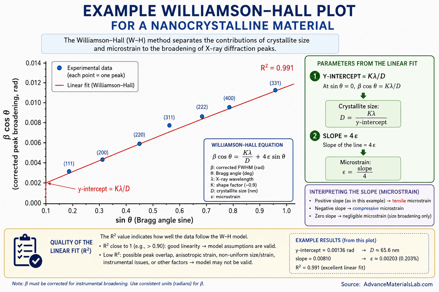
Fig. 2: Example Williamson-Hall plot for a nanocrystalline material. The x-axis shows sin θ (Bragg angle sine), and the y-axis shows β cos θ (corrected peak broadening). Each data point represents one diffraction peak. The linear regression fit (red line) yields two critical parameters: (1) the y-intercept = Kλ/D, from which crystallite size D is calculated, and (2) the slope = 4ε, from which microstrain ε is extracted. In this example, the positive slope indicates tensile microstrain. The quality of the linear fit (R² value) indicates whether the W-H model assumptions are valid for the material. | Source: AdvanceMaterialsLab.com
5.3 Interpreting Results
A successful Williamson-Hall analysis provides two quantitative outputs:
- Crystallite size D: Extracted from the intercept. Typical values: 10-100 nm for nanocrystalline materials, >200 nm for bulk materials (beyond W-H sensitivity).
- Microstrain ε: Extracted from the slope. Typical values: 10−4 to 10−2 (0.01% to 1%) for real materials. Higher strain indicates more defects, dislocations, or residual stress.
When W-H Analysis Fails
The Williamson-Hall method assumes:
- Strain is isotropic (same in all directions)
- Strain is uniformly distributed
- All peaks are pure Bragg peaks (no stacking faults, planar defects)
- Size and strain broadenings are independent
If these assumptions are violated, the W-H plot will show large scatter or physically unrealistic results (e.g., negative crystallite size). In such cases, more advanced methods like Warren-Averbach analysis or whole-pattern fitting (Rietveld refinement) are required.
6. Practical Measurement of FWHM
In this section, we discuss the practical workflow for measuring FWHM from experimental XRD data. While the concept is simple, accurate measurement requires careful attention to data quality, background subtraction, and peak fitting.
6.1 Data Collection Best Practices
- Use slow scan rates: To resolve peak shape accurately, use a scan step size of 0.01° to 0.02° (2θ) and a counting time of 2-5 seconds per step. Fast scans produce noisy peaks with unreliable FWHM.
- Ensure proper sample preparation: The sample surface should be flat and smooth. For powders, use the back-loading method or spray deposition to minimize preferred orientation. Preferred orientation can distort peak shapes and invalidate FWHM measurements.
- Use a reference standard: Measure a certified reference material (e.g., NIST SRM 660c LaB6) under identical conditions to determine instrumental broadening.
- Avoid overlapping peaks: If peaks overlap significantly, deconvolute them using multi-peak fitting before extracting FWHM. Measuring FWHM from an unresolved doublet will give meaningless results.
6.2 Background Subtraction
Accurate FWHM measurement requires proper background subtraction. The background arises from air scattering, fluorescence, and sample holder scattering. If the background is not subtracted, the measured FWHM will be artificially increased because the peak appears to start rising from a higher baseline.
Modern XRD software packages (e.g., HighScore Plus, JADE, GSAS-II) provide automated background subtraction using polynomial fitting or spline interpolation. Always visually inspect the background fit to ensure it does not cut into the peak base.
6.3 Peak Fitting Functions
XRD peaks are typically fitted to one of three mathematical profile functions:
| Function | Shape | Best For |
|---|---|---|
| Gaussian | Symmetric, exponential tails | Instrumental broadening, size broadening |
| Lorentzian | Symmetric, broader tails | Strain broadening, defect broadening |
| Voigt | Convolution of Gaussian + Lorentzian | Real peaks (combination of size and strain) |
| Pseudo-Voigt | Linear combination of Gaussian + Lorentzian | Computationally efficient approximation of Voigt |
For Scherrer and Williamson-Hall analysis, the FWHM is extracted from the fitted profile function parameters. Most software reports FWHM directly. For advanced analysis, Rietveld refinement can be used for whole-pattern fitting.
6.4 Common Errors and How to Avoid Them
- Forgetting to convert degrees to radians: The Scherrer equation requires β in radians. Always convert: β(rad) = β(deg) × π/180.
- Not correcting for instrumental broadening: Failure to subtract βinst leads to underestimated crystallite size. Always measure a reference standard.
- Using the wrong angle: The Scherrer equation uses θ (Bragg angle), which is half of the measured 2θ angle. Using 2θ instead of θ will give incorrect results.
- Applying Scherrer to strained materials: If the material has significant strain, the Scherrer equation alone is invalid. Use Williamson-Hall instead.
- Measuring FWHM from noisy or poorly fitted peaks: If the peak is noisy or the fit is poor, the FWHM will be unreliable. Improve data quality or use multi-peak fitting.
7. Worked Examples
Let us apply the concepts we have learned to real-world problems. These worked examples demonstrate the step-by-step calculation process for both the Scherrer equation and Williamson-Hall analysis.
Example 1: Calculate Crystallite Size from a Single Peak (Scherrer Equation)
Problem Statement
An XRD pattern of nanocrystalline TiO2 (rutile) shows a (110) peak at 2θ = 27.45° with FWHM βmeasured = 0.45°. The instrumental broadening βinst = 0.10° was determined using a LaB6 standard. Calculate the average crystallite size using the Scherrer equation. Assume Cu Kα radiation (λ = 0.15406 nm) and K = 0.89.
Solution:
Step 1: Correct for instrumental broadening using the Gaussian approximation:
βsample = √(0.452 − 0.102) = √(0.2025 − 0.01) = √0.1925 = 0.439°
Step 2: Convert β from degrees to radians:
Step 3: Calculate the Bragg angle θ (half of 2θ):
Step 4: Apply the Scherrer equation:
D = (0.89 × 0.15406) / (0.00766 × cos(0.2396))
D = 0.1371 / (0.00766 × 0.9718)
D = 0.1371 / 0.00744
D = 18.4 nm
Example 2: Williamson-Hall Analysis for Size and Strain Separation
Problem Statement
An XRD pattern of nanocrystalline nickel shows the following peaks after instrumental correction:
| (hkl) | 2θ (degrees) | β (radians) |
|---|---|---|
| (111) | 44.5 | 0.0052 |
| (200) | 51.8 | 0.0061 |
| (220) | 76.4 | 0.0083 |
| (311) | 92.9 | 0.0098 |
Perform a Williamson-Hall analysis to determine the crystallite size and microstrain. Use Cu Kα (λ = 0.15406 nm) and K = 0.89.
Solution:
Step 1: Calculate θ (in radians), sin θ, and β cos θ for each peak:
| (hkl) | 2θ (°) | θ (rad) | β (rad) | sin θ | β cos θ |
|---|---|---|---|---|---|
| (111) | 44.5 | 0.3886 | 0.0052 | 0.3790 | 0.00481 |
| (200) | 51.8 | 0.4524 | 0.0061 | 0.4362 | 0.00545 |
| (220) | 76.4 | 0.6668 | 0.0083 | 0.6180 | 0.00650 |
| (311) | 92.9 | 0.8113 | 0.0098 | 0.7254 | 0.00683 |
Step 2: Plot β cos θ (y-axis) vs. sin θ (x-axis) and perform linear regression. Using standard least-squares fitting, we obtain:
Intercept: 0.00395
Slope: 0.00401
Step 3: Calculate crystallite size D from the intercept:
D = Kλ / Intercept = (0.89 × 0.15406) / 0.00395
D = 0.1371 / 0.00395 = 34.7 nm
Step 4: Calculate microstrain ε from the slope:
ε = Slope / 4 = 0.00401 / 4 = 0.001003
ε = 1.00 × 10−3 = 0.10%
8. Engineering Applications of FWHM Analysis
FWHM analysis is not merely an academic exercise — it is a critical characterization tool used across multiple industries and research fields. Here are some key applications:
8.1 Nanoparticle Synthesis and Quality Control
In the synthesis of nanoparticles (catalysts, drug delivery systems, quantum dots), controlling particle size is essential. FWHM measurements provide rapid, non-destructive size characterization. For example, in the pharmaceutical industry, nanoparticle-based drug formulations are routinely characterized by XRD peak broadening to verify that the crystallite size falls within the target range (e.g., 10-50 nm for enhanced bioavailability).
8.2 Thin Film Characterization
In semiconductor manufacturing, thin films (e.g., ZnO transparent conductors, TiO2 photocatalysts) are deposited by sputtering, CVD, or ALD. The film's microstructure — crystallite size and strain — directly affects its electrical, optical, and mechanical properties. FWHM measurements track these parameters as a function of deposition conditions (temperature, pressure, substrate type), enabling process optimization.
8.3 Battery and Energy Storage Materials
In lithium-ion batteries, the cathode and anode materials undergo repeated lithiation and delithiation cycles, which induce mechanical strain and reduce crystallite size. Monitoring FWHM changes during cycling provides insight into capacity fade mechanisms. For example, broadening of the (003) peak in LiCoO2 cathodes indicates structural degradation after extended cycling.
8.4 Residual Stress Analysis in Metal Components
Machining, welding, and heat treatment introduce residual stresses in metal components. These stresses manifest as microstrain in the crystal lattice, broadening XRD peaks. Williamson-Hall analysis can quantify the microstrain, providing a non-destructive measure of residual stress. This is critical in aerospace and automotive industries, where residual stress affects fatigue life and failure resistance.
8.5 Catalysis Research
Supported metal catalysts (e.g., Pt/C, Ni/Al2O3) consist of metal nanoparticles dispersed on a high-surface-area support. The catalytic activity is strongly dependent on metal particle size — smaller particles provide higher surface area and more active sites. XRD-based crystallite size determination (via FWHM) is a standard characterization method in catalyst development.
8.6 Geological and Archaeological Studies
In mineralogy and archaeology, FWHM analysis helps determine the thermal history of materials. For example, ancient ceramics that were fired at higher temperatures have larger crystallite sizes (sharper peaks) than those fired at lower temperatures. Similarly, shock-metamorphosed minerals (from meteor impacts) show extreme peak broadening due to strain.
9. Practice Questions
Q1. The Full Width at Half Maximum (FWHM) of an XRD peak is measured at:
Q2. According to the Scherrer equation, if the FWHM of a peak doubles (increases by a factor of 2), the crystallite size:
Q3. The Scherrer equation is most accurate for crystallite sizes in the range:
Q4. In Williamson-Hall analysis, microstrain broadening increases with:
Q5. A Williamson-Hall plot with zero slope (horizontal line) indicates:
Q6. Before applying the Scherrer equation, the measured FWHM must be corrected for:
Key Takeaways — Complete Summary
- FWHM DEFINITION: Full Width at Half Maximum (β) is the angular width of an XRD peak measured at 50% of the peak's maximum intensity. It is expressed in degrees 2θ (converted to radians for calculations).
- THREE BROADENING MECHANISMS: Peak broadening arises from (1) finite crystallite size, (2) microstrain (lattice distortion), and (3) instrumental limitations. Understanding which effect dominates is essential for correct interpretation.
- CRYSTALLITE vs GRAIN SIZE: Crystallite size (from Scherrer) is the coherent diffraction domain, NOT necessarily the grain size or particle size. In mosaic crystals, one grain may contain multiple crystallites.
- SCHERRER EQUATION: D = Kλ / (β cos θ). Relates crystallite size D to FWHM β. Valid for 3-200 nm range. Assumes strain-free material. K ≈ 0.89 for spherical crystallites.
- ALWAYS CORRECT FOR INSTRUMENTAL BROADENING: Measure a reference standard (e.g., LaB6) to determine βinst, then calculate βsample = √(βmeasured2 − βinst2).
- WILLIAMSON-HALL METHOD: Separates size and strain contributions by plotting β cos θ vs. sin θ for multiple peaks. Intercept gives crystallite size; slope gives microstrain ε.
- SIZE BROADENING: βsize ∝ 1/cos θ. Affects all peaks similarly. Dominant in nanocrystalline materials.
- STRAIN BROADENING: βstrain ∝ tan θ. Increases at higher angles. Dominant in heavily deformed or defect-rich materials.
- W-H PLOT INTERPRETATION: Positive slope = tensile strain. Zero slope = strain-free (Scherrer alone sufficient). Negative slope or large scatter = model breakdown, use advanced methods.
- PRACTICAL TIPS: (1) Convert β to radians. (2) Use θ (Bragg angle), not 2θ. (3) Fit peaks with Voigt or pseudo-Voigt functions. (4) Always report K value and whether instrumental correction was applied. (5) Use W-H for strained materials; Scherrer underestimates size if strain is present.
References
All references follow IEEE citation style. All sources are peer-reviewed journals, authoritative textbooks, or internationally recognized standards.
- P. Scherrer, "Bestimmung der Größe und der inneren Struktur von Kolloidteilchen mittels Röntgenstrahlen," Nachrichten von der Gesellschaft der Wissenschaften zu Göttingen, Mathematisch-Physikalische Klasse, vol. 1918, pp. 98-100, 1918. — Original derivation of the Scherrer equation by Paul Scherrer.
- G. K. Williamson and W. H. Hall, "X-ray line broadening from filed aluminium and wolfram," Acta Metallurgica, vol. 1, no. 1, pp. 22-31, Jan. 1953, doi: 10.1016/0001-6160(53)90006-6. [DOI] — Seminal paper introducing the Williamson-Hall method for separating size and strain broadening.
- B. D. Cullity and S. R. Stock, Elements of X-Ray Diffraction, 3rd ed. Upper Saddle River, NJ, USA: Pearson Prentice Hall, 2001, ch. 9-10. — Definitive textbook covering peak broadening analysis, Scherrer equation, and Williamson-Hall method with worked examples.
- H. P. Klug and L. E. Alexander, X-Ray Diffraction Procedures for Polycrystalline and Amorphous Materials, 2nd ed. New York, NY, USA: Wiley, 1974, ch. 9. — Classic reference on line profile analysis and crystallite size determination.
- J. I. Langford and A. J. C. Wilson, "Scherrer after sixty years: A survey and some new results in the determination of crystallite size," Journal of Applied Crystallography, vol. 11, no. 2, pp. 102-113, Apr. 1978, doi: 10.1107/S0021889878012844. [DOI] — Comprehensive review of the Scherrer equation, shape factors, and validity limits.
- A. L. Patterson, "The Scherrer formula for X-ray particle size determination," Physical Review, vol. 56, no. 10, pp. 978-982, Nov. 1939, doi: 10.1103/PhysRev.56.978. [DOI] — Early theoretical analysis of the Scherrer equation and its physical meaning.
- R. A. Young, Ed., The Rietveld Method. New York, NY, USA: Oxford University Press, 1993. — Reference for advanced whole-pattern fitting methods that supersede simple Scherrer analysis for complex materials.
- M. A. Krivoglaz, X-Ray and Neutron Diffraction in Nonideal Crystals. Berlin, Germany: Springer-Verlag, 1996. — Advanced theoretical treatment of diffraction line broadening mechanisms including strain, dislocations, and stacking faults.
- International Union of Crystallography (IUCr), "Commission on Powder Diffraction Newsletter No. 26," IUCr CPD Newsletter, 2001. [IUCr Online] — Guidelines for accurate FWHM measurement and instrumental broadening correction.
- National Institute of Standards and Technology (NIST), "Standard Reference Material 660c — Lanthanum Hexaboride Powder Line Position and Line Shape Standard for Powder Diffraction," NIST SRM 660c Certificate. [NIST Certificate] — Official NIST reference standard for instrumental broadening calibration.
- U. Holzwarth and N. Gibson, "The Scherrer equation versus the 'Debye-Scherrer equation'," Nature Nanotechnology, vol. 6, no. 9, pp. 534-534, Sep. 2011, doi: 10.1038/nnano.2011.145. [DOI] — Historical note clarifying the correct attribution of the Scherrer equation.
- A. Monshi, M. R. Foroughi, and M. R. Monshi, "Modified Scherrer equation to estimate more accurately nano-crystallite size using XRD," World Journal of Nano Science and Engineering, vol. 2, no. 3, pp. 154-160, 2012, doi: 10.4236/wjnse.2012.23020. [DOI] — Discussion of instrumental correction methods and shape factor selection for nanocrystals.